10-1100/Assignment 1 Part 1 by Peter
Pyraminx Analysis Using Matlab
By: Peter Badea
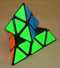
This article will attempt to guide the reader through an analysis of the number of possible permutations of a Pyraminx puzzle (see Pyraminx):
Please Note: It has come to my attention that Mr. Charles Tsang has also posted an analysis of the Pyraminx problem. This is an unfortunate coincidence that was only observed after the problem had been solved. A quick glance at the very different program code (and even program used) will surely lead any reader to this conclusion. His solution can be found here.
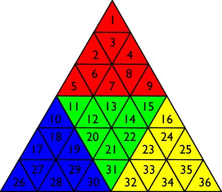
As can be seen above, this puzzle is similar to that of the Rubik's cube except for the differing shape (that of a tetrahedron as opposed to a cube). Each side is an equilateral triangle composed of 9 smaller equilateral triangles all joined in the fashion shown below:
The labeling shown above is important to understand the meaning of each permutation expressed in standard notation. To apply the the Schreier–Sims algorithm to this problem, a set of generators must first be found. These can be expressed as the 8 rotations (about each of 4 vertices) that involve rotating either only the vertex piece (4 trivial rotations) or 2 (of the total 3) rows of pieces.
A recursive function for feeding each permutation into the table T is then constructed in Matlab:
   function Tnew = feed(s,T)

   j2 = 0;
   Tnew = T;

   %find pivot point
   for i2 = 1:36
       if s(i2) ~= i2
           j2 = s(i2);
           break
       end
   end

   if j2 ~= 0 %s is not identity permutation
       if T(1,i2,j2) == 0 %empty box
           Tnew(:,i2,j2) = s;
       else %T(1,i2,j2) ~= 0; non-empty box
           for k2 = 1:36 %define t inverse, where t is the permutation currently in the box
               tInv(k2) = find(T(:,i2,j2) == k2);
           end

           for k2 = 1:36 %define t inverse * s
               tInvs(k2) = tInv(s(k2));
           end

           %feed t inverse * s
           Tnew = feed(tInvs,T);
   end

   end
Using this function, the Schreier–Sims algorithm is then implemented in Matlab in the following way:
   clear
   clc

   T = zeros(36,36,36);

   %initialize T
   for i = 1:36
       T(:,i,i) = ones(36,1);
   end

   Tnew = T;

   %generators
   s1 = 1:36;
   s1([1,26,36]) = [26,36,1];

   s2 = 1:36;
   s2([5,10,11]) = [10,11,5];

   s3 = 1:36;
   s3([9,15,16]) = [15,16,9];

   s4 = 1:36;
   s4([30,31,32]) = [31,32,30];

   s5 = 1:36;
   s5([2,3,4,17,25,27,28,34,35]) = [28,27,17,34,2,35,25,4,3];

   s6 = 1:36;
   s6([2,6,7,12,13,17,18,19,20]) = [13,12,20,18,19,7,6,2,17];

   s7 = 1:36;
   s7([4,7,8,13,14,22,23,24,25]) = [13,22,14,23,24,25,4,8,7];

   s8 = 1:36;
   s8([19,20,21,22,23,28,29,33,34]) = [22,23,33,34,28,20,21,29,19];

   %feed generators into Tnew
   Tnew = feed(s1,Tnew);
   Tnew = feed(s2,Tnew);
   Tnew = feed(s3,Tnew);
   Tnew = feed(s4,Tnew);
   Tnew = feed(s5,Tnew);
   Tnew = feed(s6,Tnew);
   Tnew = feed(s7,Tnew);
   Tnew = feed(s8,Tnew);

   while length(find(Tnew ~= T)) ~= 0 %while table is still changing
       T = Tnew;
       for i = 1:35
           for j = i+1:36
               for k = 1:35
                   for l = k+1:36
                       if T(1,i,j) ~= 0 & T(1,k,l) ~= 0
                           Tnew = feed(T(T(:,k,l),i,j),Tnew);
                       end
                   end
               end
           end
       end
   end

   ord = 1;

   for i = 1:36
       ord = ord * length(find(T(1,i,:)));
   end

   disp(['Order = ',num2str(ord)])

   for i = 1:36
       for j = 1:36
           if T(1,i,j) ~= 0
               plot(i,j,'+')
               hold on
               axis equal
           end
       end
   end
The above code yields the following result:
Order = 75582720
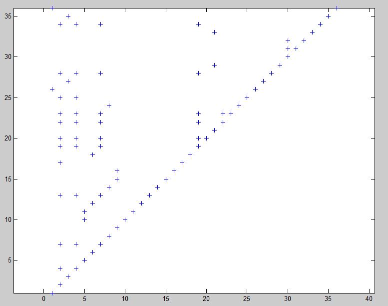
Graphing the values where the table T is non-zero yields the following graph:

If we then change the code slightly to disallow turning of the 4 vertex pieces (the trivial rotations), we get a different result:
Order = 933120
This is a more accurate description of the difficulty that solving such a puzzle would entail due to the fact that the 4 vertex pieces may always be turned at the very end, and no particular strategy needs to be employed in placing them.

