User:Zsuzsi/HW4
The Generators
Our generators are [math]\displaystyle{ T }[/math], [math]\displaystyle{ R }[/math], [math]\displaystyle{ \Phi }[/math] and [math]\displaystyle{ B^{\pm} }[/math]:
A low-tech completed version of this chart:
The Relations
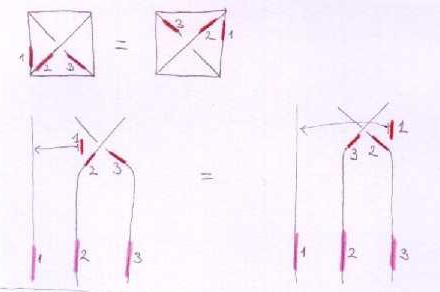
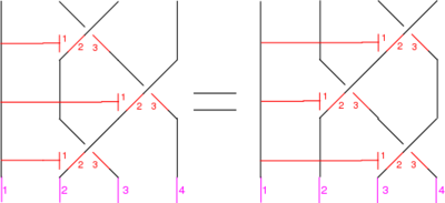
The Symmetry of B
To eliminate the choice involved in placing a B at a crossing, it has to have 180 degrees rotational symmetry. This yields the following picture:
The relation cannot be written in the first notation, as on the right side the chords ending on different red lines could end up on the same pink line.
In the linearized functional notation though we can express this:
[math]\displaystyle{ s_1(x_1,x_2,x_3)=b^+(x_1,x_2,x_3)-b^+(-x_1-x_2-x_3,-x_3,-x_2) }[/math]
Explanation: on the right side, chords on the first red line can drop off on either the third, second or the first strand, morover, the orders are reversed, hence the minus signs.
The same picture for B^- yields:
[math]\displaystyle{ s_2(x_1,x_2,x_3)=b^-(x_1,x_2,x_3)-b^-(-x_1-x_2-x_3,-x_3,-x_2) }[/math]
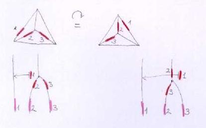
The symmetry of [math]\displaystyle{ \Phi }[/math]
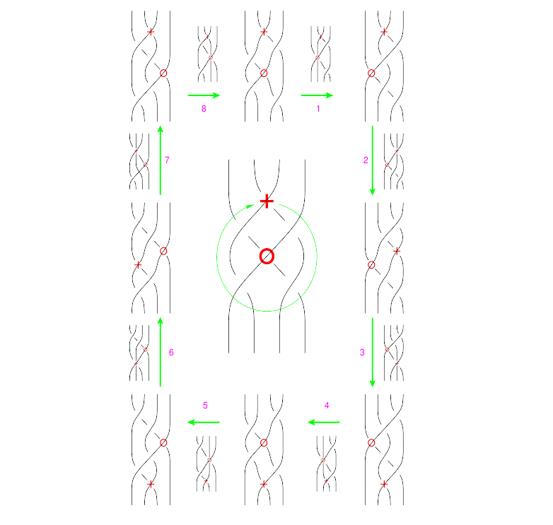
[math]\displaystyle{ \Phi }[/math] has to have A(4)-symmetry. For example, rotation around the "top" vertex yields the following picture and relation:
The same explanation goes here, and we get the relation:
[math]\displaystyle{ s_3(x_1,x_2,x_3)=\varphi(x_1,x_2,x_3)-\varphi(-x_1-x_2,-x_2-x_3,x_2) }[/math]
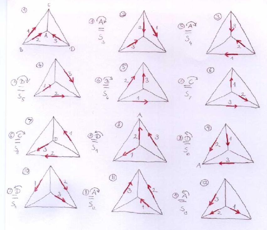
And here is the full picture and the relations (I suppose it would be enough to take a few that generate A(4), but we're on the safe side writing all these up... and I kind of got into drawing tetrahedrons.):
[math]\displaystyle{ s_3(x_1,x_2,x_3)=\varphi(x_1,x_2,x_3)-\varphi(-x_1-x_2,-x_2-x_3,x_2) }[/math]
[math]\displaystyle{ s_4(x_1,x_2,x_3)=\varphi(-x_1-x_2,-x_2-x_3,x_2)-\varphi(x_1+x_2,x_3,-x_2-x_3) }[/math]
[math]\displaystyle{ s_5(x_1,x_2,x_3)=\varphi(x_1+x_2,x_3,-x_2-x_3)-\varphi(x_2,-x_1-x_2,x_1+x_2+x_3) }[/math]
[math]\displaystyle{ s_6(x_1,x_2,x_3)=\varphi(x_2,-x_1-x_2,x_1+x_2+x_3)-\varphi(-x_1-x_2,x_1,x_2+x_3) }[/math]
[math]\displaystyle{ s_7(x_1,x_2,x_3)=\varphi(-x_1-x_2,x_1,x_2+x_3)-\varphi(x_2+x_3,-x_3,-x_1-x_2) }[/math]
[math]\displaystyle{ s_8(x_1,x_2,x_3)=\varphi(x_2+x_3,-x_3,-x_1-x_2)-\varphi(-x_1-x_2-x_3,-x_2,x_1+x_2) }[/math]
[math]\displaystyle{ s_9(x_1,x_2,x_3)=\varphi(-x_1-x_2-x_3,-x_2,x_1+x_2)-\varphi(-x_2,x_2+x_3,-x_1-x_2-x_3) }[/math]
[math]\displaystyle{ s_{10}(x_1,x_2,x_3)=\varphi(-x_2,x_2+x_3,-x_1-x_2-x_3)-\varphi(-x_2-x_3,-x_1,x_1+x_2) }[/math]
[math]\displaystyle{ s_{11}(x_1,x_2,x_3)=\varphi(-x_2-x_3,-x_1,x_1+x_2)-\varphi(-x_1,x_1+x_2+x_3,-x_3) }[/math]
[math]\displaystyle{ s_{12}(x_1,x_2,x_3)=\varphi(-x_1,x_1+x_2+x_3,-x_3)-\varphi(x_3,-x_1-x_2-x_3,x_1) }[/math]
[math]\displaystyle{ s_{13}(x_1,x_2,x_3)=\varphi(x_3,-x_1-x_2-x_3,x_1)-\varphi(-x_3,-x_2,-x_1) }[/math]
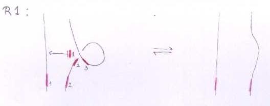
The Reidemeister move R1
As with the symmetry relations, we cannot write this one in the first notation either.
In the linearized functional notation, it looks like this:
[math]\displaystyle{ \rho_1(x_1,x_2)=b^-(x_1,x_2,-x_2) }[/math]
Where the negative sign is because the order of the chords is reversed as we slide them along the little loop.
The Reidemeister move R2
With three sides of the shielding removed, the picture is:
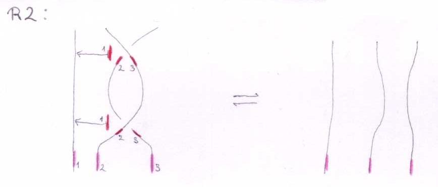
This means: [math]\displaystyle{ (123)^\star B^+ (132)^\star B^- = 1 }[/math]
Linearized and in functional form:
[math]\displaystyle{ \rho_2(x_1,x_2,x_3)=b^+(x_1,x_2,x_3)+b^-(x_1,x_3,x_2) }[/math]
And we get the other R2 by switching both crossings, i.e. switching b^+ and b^-:
[math]\displaystyle{ \rho_2'(x_1,x_2,x_3)=b^-(x_1,x_2,x_3)+b^+(x_1,x_3,x_2) }[/math]
The Reidemeister Move R3
The picture (with three sides of the shielding removed) is
In formulas, this is
Linearized and written in functional form, this becomes
| [math]\displaystyle{ \rho_3(x_1, x_2, x_3, x_4) = }[/math] | [math]\displaystyle{ b^+(x_1,x_2,x_3) + b^+(x_1+x_3,x_2,x_4) + b^+(x_1,x_3,x_4) }[/math] |
| [math]\displaystyle{ - b^+(x_1+x_2,x_3,x_4) - b^+(x_1,x_2,x_4) - b^+(x_1+x_4,x_2,x_3). }[/math] |
The Reidemeister Move R4, source:Andy
First version of R4:
In formulas, this is
Linearized and written in functional form, this becomes
| [math]\displaystyle{ \rho_{4a}(x_1,x_2,x_3,x_4) = b^+(x_1,x_2,x_3) + b^+(x_1+x_3,x_2,x_4) + \phi(x_1,x_3,x_4) - \phi(x_1+x_2,x_3,x_4) - b^+(x_1,x_2,x_3+x_4). }[/math] |
Second version:
In formulas, this is
Linearized and written in functional form, this becomes
| [math]\displaystyle{ \rho_{4b}(x_1,x_2,x_3,x_4) = b^+(x_1+x_2,x_3,x_4) + b^+(x_1,x_2,x_4) + \phi(x_1+x_4,x_2,x_3) - \phi(x_1,x_2,x_3) - b^+(x_1,x_2+x_3,x_4). }[/math] |
The Syzygies
The "B around B" Syzygy
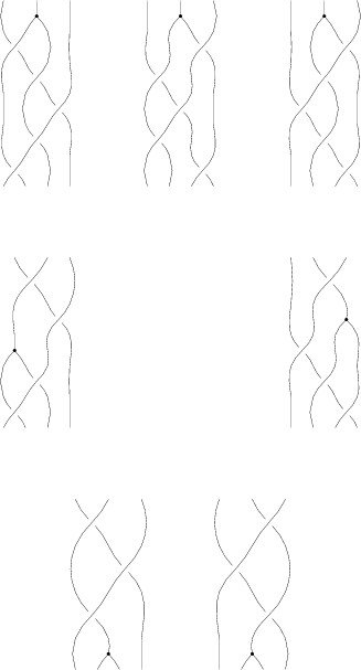
The picture, with all shielding removed, is
| (Drawn with Inkscape) (note that lower quality pictures are also acceptable) |
The functional form of this syzygy is
| [math]\displaystyle{ BB(x_1,x_2,x_3,x_4,x_5) = }[/math] | [math]\displaystyle{ \rho_3(x_1, x_2, x_3, x_5) + \rho_3(x_1 + x_5, x_2, x_3, x_4) - \rho_3(x_1 + x_2, x_3, x_4, x_5) }[/math] |
| [math]\displaystyle{ - \rho_3(x_1, x_2, x_4, x_5) - \rho_3(x_1 + x_4, x_2, x_3, x_5) - \rho_3(x_1, x_2, x_3, x_4) }[/math] | |
| [math]\displaystyle{ + \rho_3(x_1, x_3, x_4, x_5) + \rho_3(x_1 + x_3, x_2, x_4, x_5). }[/math] |
The "[math]\displaystyle{ \Phi }[/math] around B" Syzygy- I copy-pasted this from Andy, as well as R4
The picture, with all shielding (and any other helpful notations) removed, is
| (Drawn with Asymptote, Syzygies in Asymptote) |
The functional form of this syzygy is
| [math]\displaystyle{ \Phi B(x_1,x_2,x_3,x_4,x_5) = }[/math] | [math]\displaystyle{ \rho_3(x_1,x_2,x_3,x_5) + \rho_{4a}(x_1+x_5,x_2,x_3,x_4) + \rho_{4b}(x_1+x_2,x_3,x_4,x_5) }[/math] |
| [math]\displaystyle{ - \rho_3(x_1,x_2,x_3+x_4,x_5) - \rho_{4a}(x_1,x_2,x_3,x_4) }[/math] | |
| [math]\displaystyle{ - \rho_{4b}(x_1,x_3,x_4,x_5) + \rho_3(x_1+x_3,x_2,x_4,x_5). }[/math] |
The "[math]\displaystyle{ \Phi }[/math] around [math]\displaystyle{ \Phi }[/math]" Syzygy -also taken from Andy
note: I've changed Andy's notation to fit my version of R2.
The picture is
| (Drawn with Asymptote, Syzygies in Asymptote) |
The functional form of this syzygy is
| [math]\displaystyle{ \Phi\Phi(x_1,x_2,x_3,x_4,x_5) = }[/math] | [math]\displaystyle{ -\rho_2'(x_1+x_2,x_3,x_4) - \rho_2'(x_1+x_2+x_4,x_3,x_5) + \rho_{4b}(x_1+x_2,x_4,x_5,x_3) }[/math] |
| [math]\displaystyle{ - \rho_2'(x_1,x_2,x_4) - \rho_2'(x_1+x_4,x_2,x_5) + \rho_{4b}(x_1,x_4,x_5,x_2) }[/math] | |
| [math]\displaystyle{ + \rho_{4a}(x_1,x_4+x_5,x_2,x_3) - \rho_{4b}(x_1,x_4,x_5,x_2+x_3) - \rho_{4a}(x_1+x_4,x_5,x_2,x_3) }[/math] | |
| [math]\displaystyle{ + \rho_2'(x_1+x_4,x_2,x_5) + \rho_2'(x_1+x_2+x_4,x_3,x_5) - \rho_{4a}(x_1,x_4,x_2,x_3) }[/math] | |
| [math]\displaystyle{ + \rho_2'(x_1,x_2,x_4) + \rho_2'(x_1+x_2,x_3,x_4) }[/math] |
Note that the first and last terms cancel, as the two steps at the top of the diagram are opposites.
A Mathematica Verification
The following simulated Mathematica session proves that for our single relation and single syzygy, [math]\displaystyle{ d^2=0 }[/math]. Copy paste it into a live Mathematica session to see that it's right!
In[1]:=
|
d1 = {
  rho3[x1_, x2_, x3_, x4_] :> bp[x1, x2, x3] + bp[x1 + x3, x2, x4] +
  bp[x1, x3, x4] - bp[x1 + x2, x3, x4] - bp[x1, x2, x4] -
  bp[x1 + x4, x2, x3]
};
d2 = {
  BAroundB[x1_, x2_, x3_, x4_, x5_] :> rho3[x1, x2, x3, x5] +
  rho3[x1 + x5, x2, x3, x4] - rho3[x1 + x2, x3, x4, x5] -
  rho3[x1, x2, x4, x5] - rho3[x1 + x4, x2, x3, x5] -
  rho3[x1, x2, x3, x4] + rho3[x1, x3, x4, x5] +
  rho3[x1 + x3, x2, x4, x5]
};
|
In[3]:=
|
BAroundB[x1, x2, x3, x4, x5] /. d2
|
Out[3]=
|
- rho3[x1, x2, x3, x4] + rho3[x1, x2, x3, x5] - rho3[x1, x2, x4, x5]
+ rho3[x1, x3, x4, x5] - rho3[x1 + x2, x3, x4, x5]
+ rho3[x1 + x3, x2, x4, x5] - rho3[x1 + x4, x2, x3, x5]
+ rho3[x1 + x5, x2, x3, x4]
|
In[4]:=
|
BAroundB[x1, x2, x3, x4, x5] /. d2 /. d1
|
Out[4]=
|
0
|


