User:Shawkm/06-1350-HW4
The Generators
Our generators are [math]\displaystyle{ T }[/math], [math]\displaystyle{ R }[/math], [math]\displaystyle{ \Phi }[/math] and [math]\displaystyle{ B^{\pm} }[/math]:
The Relations
The Reidemeister Move R3
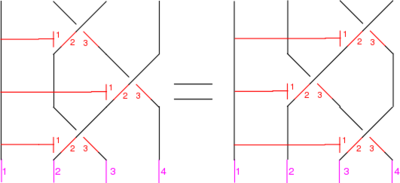
The picture (with three sides of the shielding removed) is
In formulas, this is
Linearized and written in functional form, this becomes
| [math]\displaystyle{ \rho_3(x_1, x_2, x_3, x_4) = }[/math] | [math]\displaystyle{ b^+(x_1,x_2,x_3) + b^+(x_1+x_3,x_2,x_4) + b^+(x_1,x_3,x_4) }[/math] |
| [math]\displaystyle{ - b^+(x_1+x_2,x_3,x_4) - b^+(x_1,x_2,x_4) - b^+(x_1+x_4,x_2,x_3). }[/math] |
The Syzygies
The "B around B" Syzygy
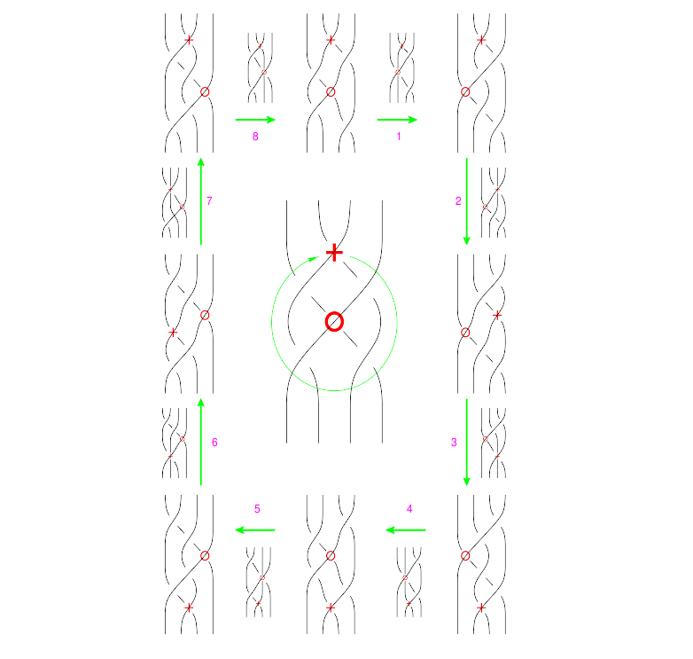
The picture, with all shielding removed, is
| (Drawn with Inkscape) (note that lower quality pictures are also acceptable) |
The functional form of this syzygy is
| [math]\displaystyle{ BB(x_1,x_2,x_3,x_4,x_5) = }[/math] | [math]\displaystyle{ \rho_3(x_1, x_2, x_3, x_5) + \rho_3(x_1 + x_5, x_2, x_3, x_4) - \rho_3(x_1 + x_2, x_3, x_4, x_5) }[/math] |
| [math]\displaystyle{ - \rho_3(x_1, x_2, x_4, x_5) - \rho_3(x_1 + x_4, x_2, x_3, x_5) - \rho_3(x_1, x_2, x_3, x_4) }[/math] | |
| [math]\displaystyle{ + \rho_3(x_1, x_3, x_4, x_5) + \rho_3(x_1 + x_3, x_2, x_4, x_5). }[/math] |
A Mathematica Verification
The following simulated Mathematica session proves that for our single relation and single syzygy, [math]\displaystyle{ d^2=0 }[/math]. Copy paste it into a live Mathematica session to see that it's right!
In[1]:=
|
d1 = {
  rho3[x1_, x2_, x3_, x4_] :> bp[x1, x2, x3] + bp[x1 + x3, x2, x4] +
  bp[x1, x3, x4] - bp[x1 + x2, x3, x4] - bp[x1, x2, x4] -
  bp[x1 + x4, x2, x3]
};
d2 = {
  BAroundB[x1_, x2_, x3_, x4_, x5_] :> rho3[x1, x2, x3, x5] +
  rho3[x1 + x5, x2, x3, x4] - rho3[x1 + x2, x3, x4, x5] -
  rho3[x1, x2, x4, x5] - rho3[x1 + x4, x2, x3, x5] -
  rho3[x1, x2, x3, x4] + rho3[x1, x3, x4, x5] +
  rho3[x1 + x3, x2, x4, x5]
};
|
In[3]:=
|
BAroundB[x1, x2, x3, x4, x5] /. d2
|
Out[3]=
|
- rho3[x1, x2, x3, x4] + rho3[x1, x2, x3, x5] - rho3[x1, x2, x4, x5]
+ rho3[x1, x3, x4, x5] - rho3[x1 + x2, x3, x4, x5]
+ rho3[x1 + x3, x2, x4, x5] - rho3[x1 + x4, x2, x3, x5]
+ rho3[x1 + x5, x2, x3, x4]
|
In[4]:=
|
BAroundB[x1, x2, x3, x4, x5] /. d2 /. d1
|
Out[4]=
|
0
|
Here Goes Something New(?)
The first thing to notice is that the relation [math]\displaystyle{ \rho_3 }[/math] holds for [math]\displaystyle{ b^+ }[/math] and [math]\displaystyle{ b^- }[/math] so we have another version:
| [math]\displaystyle{ \rho_3(x_1, x_2, x_3, x_4) = }[/math] | [math]\displaystyle{ b^-(x_1,x_2,x_3) + b^-(x_1+x_3,x_2,x_4) + b^-(x_1,x_3,x_4) }[/math] |
| [math]\displaystyle{ - b^-(x_1+x_2,x_3,x_4) - b^-(x_1,x_2,x_4) - b^-(x_1+x_4,x_2,x_3). }[/math] |
This is probably a completely trivial remark, and it is also trivial to see that mathematica will deal with this in the same way as for [math]\displaystyle{ b^+ }[/math] so I won't verify that [math]\displaystyle{ d^2 =0 }[/math].
What I will do now is linearize and write down in functional form the relation R2
| [math]\displaystyle{ \rho_2(x_1, x_2, x_3) = }[/math] | [math]\displaystyle{ b^+(x_1,x_2,x_3) + b^-(x_1,x_3,x_2) }[/math] |
or
| [math]\displaystyle{ \rho_2(x_1, x_2, x_3) = }[/math] | [math]\displaystyle{ b^-(x_1,x_2,x_3) + b^+(x_1,x_3,x_2) }[/math] |


